Week 10: Matrices and Evolutionary Algorithms

Readings

Since we're moving to shorter class sessions, it's really important that you do the readings and exercises before the class session. Every class will start with a prompt to come up with three questions based on the reading material.

Session 1

Session 2

Kate Compton, "Let it Grow: Practical Procedural Generation from the Ground Up"
What is an Evolutionary Algorithm?, section 2.1 up to but not including 2.4. It's okay to read it and not understand it all: we're just reading for vocabulary and the high level structure.

Key Questions

How do I create and access elements of a nested list?
How do I iterate over a nested list, to produce either a single value or another nested list?
Where would I choose to use a nested list of lists?
What are the key components of an evolutionary algorithm?
How are evolutionary algorithms like and unlike the biological process that inspired them?
Where are evolutionary algorithms useful and where might they be less useful?

Topics

Lists of lists (matrices)

What is a matrix?

A two-dimensional data structure which is rectangular
```
0 1 0
1 8 2
5 0 3
```
- Some number of columns; every row has the same number of elements.
- The second row: 1 8 2
- The third column: 0 2 3
- We'll use 0-indices again, so matrix[1] gives us the second row
- How do we get the middle element?
  - matrix[1][1] (row 1, col 1)

How can we implement it in Python?

A matrix is a list of lists!

>>> m = [[0, 1, 0], [1, 8, 2], [5, 0, 3]]
>>> m
[[0, 1, 0], [1, 8, 2], [5, 0, 3]]
>>> m[1][2]
2
>>> m[2][2]
3

Or:

>>> m = []
>>> m.append([0, 1, 0])
>>> m.append([1, 8, 2])
>>> m.append([5, 0, 3])
>>> m
[[0, 1, 0], [1, 8, 2], [5, 0, 3]]
>>> m[1][2]
2
>>> m[2][2]
3

So m[1] is the second row
The second column would be [m[0][1], m[1][1], m[2][1]]
- Kind of awkward! Libraries like numpy make this smoother and allow the use of slicing syntax.

matrix.py

What do zero_matrix and zero_matrix2 do?

They create zeroed-out matrices of the given dimensions
zero_matrix works one entry at a time

zero_matrix2 does it a row at a time

>>> zero_matrix(3)
[[0, 0, 0], [0, 0, 0], [0, 0, 0]]
>>> zero_matrix(2)
[[0, 0], [0, 0]]
>>> zero_matrix(1)
[[0]]
>>> m = zero_matrix(2)
>>> m[1][1] = 100
>>> m
[[0, 0], [0, 100]]

What does random_matrix do?

Same thing, but with random numbers:

>>> random_matrix(3)
[[7, 9, 9], [3, 6, 6], [6, 6, 2]]
>>> random_matrix(3)
[[9, 5, 8], [1, 2, 3], [8, 9, 8]]
>>> random_matrix(3)
[[1, 0, 0], [4, 3, 8], [2, 7, 7]]

When we print out a matrix we get that list of lists representation
- How could we print it out a row at a time?
- Well, we iterate through the rows!
- Check out print_matrix
What does the identity function do?
- Creates an identity matrix, i.e. all zeros except for ones along the diagonal
How could we sum up the numbers in a matrix?
- Iterate through each entry (two nested for loops)
  - How many rows? len(mat). How many columns? len(mat[0]) (it had better be equal to len(mat[1]), etc!
- Or iterate through the rows and use sum()
- Check out matrix_sum through matrix_sum4 for alternatives

Using matrices

Lots of board games happen on discrete grids
- These could be represented with a matrix!
Check out tic_tac_toe.py
- How might you represent a tic-tac-toe (noughts and crosses) board?
- A 3x3 matrix!
  - Not of numbers, though: of "_", "X", or "O"
  - Or None, "X", "O"
  - Or -1, 0, 1?
  - Or class Nought, class Cross, class Empty?
  - Or class TTTSpot?
  - Lots of options
- Look at __init__ and is_goal. What do these do and how do they work?
  - Is is_goal correct?
Challenge problem: how would you copy a tic tac toe board two times, so you could try out two different moves without necessarily committing to either one? This series of steps should work perfectly:
- Make two copies of the board
- Make a move in copy 1 (make sure copy 2 and original don't change!)
- Make a move in copy 2 (make sure copy 1 and original don't change!)
- How did you solve it?

`numpy`

numpy is a Python module for efficient computations with numeric data. It can be installed via pip, like we did for PyTorch in the neural network lab. Its main idea is the "n-dimensional array", a generalization of matrices. The primary motivations for using numpy rather than just lists of lists of (lists of lists of…) numbers are:

No chance of accidentally having a wrongly-sized row or whatever! Numpy guarantees that the shape is consistent and rectangular.
A large suite of mathematical functions: everything from linear algebra to stats and beyond.
Extremely efficient implementation of n-dimensional arrays.

This last point is possible primarily due to differences in data structures. Consider that a Python list of lists would have a structure in memory like this:

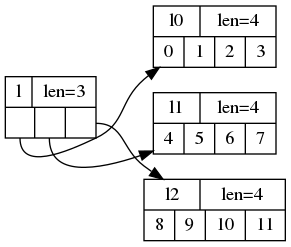
Each of those list objects (l, l0, l1, l2) is its own memory allocation, and l's entries are just pointers to each row. This means that to find l[1][2], we first need to find the second row from l, look that up in memory, and then find the third column. Even worse, Python lists can store any type of value (and a mix of them!), which is less efficient than having them be specialized for storing just numbers of a particular type.

Compare numpy's internal representation:

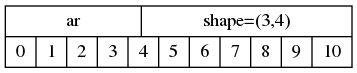
Here, one allocation is used and when we want the second row and third column we write ar[1,3]—it's easy to compute exactly where in memory this is and go right there. Note that we're not using two sets of square braces, but one set of square braces with a tuple as the index (numpy accepts either way, but the tuple version is more idiomatic). Some more examples:

>>> import numpy
>>> arr = numpy.zeros(shape=(3,2))
>>> arr
array([[0., 0.],
       [0., 0.],
       [0., 0.]])
>>> arr[0] # Get the first row
array([0., 0.])
>>> arr[0] = (1,2) # Set each element of the first row according to the given sequence
>>> arr
array([[1., 2.], # Look, we set two values at once!
       [0., 0.],
       [0., 0.]])
>>> arr[1][1] = 7 # Set a specific index
>>> arr[1,0] = 6 # Same here
>>> arr
array([[1., 2.],
       [6., 7.],
       [0., 0.]])
>>> arr[:, 0] = 47 # We can also set a whole column at once!
>>> arr
array([[47.,  2.],
       [47.,  7.],
       [47.,  0.]])

Numpy's particular use of the slicing syntax is part of what makes it so pleasant to use:

The third row of an array: arr[4].
The fourth column of an array: arr[3, :].
The middle four elements of a 4x4 array, as a 2x2 array: arr[1:3,1:3].

This generalizes to three and more dimensions. For example, we might represent an image as a height-by-width-by-RGB array:

# Here's a 16x16x3 red square:
red = numpy.zeros(shape=(16,16,3))
red[:,:,0] = 1.0 # We usually use 0.0 to 1.0 as the range for color components
# everything else is zeros!

blue_square = numpy.array(red) # Make a copy of red
blue_square[0:4, 0:4, :] = (0,0,1.0) # Make a blue square in the top left

Note that even slices of numpy arrays are aliases:

ones = numpy.ones(shape=(2,2))
col0 = ones[:,0]
print(col0.shape) # (2,)
col0[:] = 2
print(col0) #[2. 2.]
print(ones)
# [[2. 1.]  # Whoops, first column is now 2s!
#  [2. 1.]]

Numpy is used widely in scientific computing and the sciences.

picture.py

The picture module is something you'll be using in assignment 9. The example we'll be discussing here is a trimmed down version.

Check out the key methods of the Picture class, which wraps a numpy array:

clear—Clears out the picture to be fully black
compare—Calculates the sum of squared differences between two pictures. This is a measure of how different the two pictures are.
write_ppm—Writes out the picture as a ppm format image file. The main step here is converting the pixel data from the [0,1] range to the [0,255] range and outputting them as unsigned 8-bit integers instead of floating point numbers.
blend_rect—Given a rectangle (xywh) and a color (rgba), draw the rectangle "blended" (or "composited") on top of the picture (instead of just replacing the existing color with the new color). Check out the two question comments in blend_rect and see if you can answer them!

Evolutionary Algorithms

Evolutionary algorithms, also called genetic algorithms, are inspired by the biological processes of natural selection and cross-breeding. Because we're working on computers and not cells, we need to come up a suitable abstraction for these processes. Usually, we imagine that our population is a collection (maybe a list) of individuals, and each individual has a genome made up of some numbers (maybe a list of numbers or maybe an array of bits).

We simulate natural selection by rating individuals according to their fitness—a function we come up with to go from an individual (i.e., a genome) and possibly an environment to a numerical score. This numerical score is how "good" this individual is. Once we know the quality of each individual, we can use some selection strategy to pick pairs of individuals whose genes we want to cross over to produce new individuals. During crossover, some genes of each "parent" are chosen to produce one or more offspring. Often, these new individuals are mutated in place to introduce more genetic diversity.

Successful evolutionary algorithms manage the conflict between wanting good-quality individuals (to solve the problem under consideration) with wanting a diverse population of individuals (to draw new genetic material from). They can be very effective if it's easier to explain why a candidate solution is good than it is to tweak a candidate solution to make it better.

Here's the pseudocode template for doing a genetic algorithm:

def evolve_step(population):
    new_pop = []
    new_pop += keep_some(population)
    while want_more_offspring:
        ind1, ind2 = select_two(population)
        ind = spawn_offspring(ind1, ind2)
        mutate(ind)
        new_pop.append(ind)
    while want_more_random:
        new_pop.append(new_random_individual())
    sort_by_fitness(new_pop)
    return new_pop

def ga(steps):
    pop = initial_population()
    for step in range(steps):
        pop = evolve_step(pop)
        if stopping_criterion(pop):
            break
    return pop

Evolving bad guys by hand

Since homework 9 uses an automatic selection criterion, let's explore a more "unnatural" selection: personal taste!

We'll evolve cool looking monsters in the style of Space Invaders:

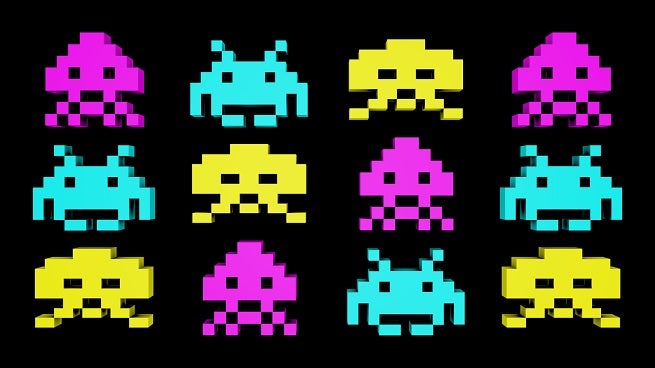
These guys have horizontal symmetry, and they're a single color, and they're 8x8 pixels large. So we only need to evolve their left halves and reflect that to obtain the image for the right half.

import numpy
class Monster:
    def __init__(self):
        # A bunch of random booleans
        self.pixels = numpy.random.randint(0,2,size=(8,4)) # 8 rows by 4 columns
    def to_picture(self, color):
        # A bunch of numpy-fu to turn 8x4 into 8x4x3 wherever colors is 1
        full = numpy.hstack((self.pixels, self.pixels[:,::-1]))
        colors = full[:,:,numpy.newaxis]
        colors = color*colors
        # This would also work:
        # colors = numpy.zeros(shape=(8,8,3))
        # colors[numpy.nonzeros(full)] = color
        return colors

Now, we could easily draw monsters into files by creating a Picture and using its write_ppm method. We also have two more methods to Monster to handle crossover and mutation. (See evol.py to follow along.)

In crossover_with we use a technique called "single point crossover". We could instead arbitrarily pick each pixel from self or mon2, or we could pick each row or column arbitrarily from one or the other. mutate uses a variety of mutation options as well: uniform mutation (every pixel might toggle), vertical flipping, or horizontal flipping.

evol.py draws a bunch of monsters on the screen and lets the user click to select a pair to breed (the ones the user likes best perhaps). Then we just apply the genetic operators of crossover and mutation to come up with new examples! It's worth looking deeply at this code; we'll also build it up in pieces during the week's second lecture.